Working on my Bachelor Thesis[5], I noticed that several authors have trained a Partially Observable Markov Decision Process (POMDP) using a variant of the Baum-Welch Procedure (for example McCallum [4][3]) but no one actually gave a detailed description how to do it. In this post I will highlight some of the difficulties and present a possible solution based on an idea proposed by Devijver [2]. In the first part I will briefly present the Baum-Welch Algorithm and define POMDPs in general. Subsequently, a version of the alpha-beta algorithm tailored to POMDPs will be presented from which we can derive the update rule. Finally I will present a sample implementation in Python. If you are not interested in the theory, just skip over to the last part.
The Baum-Welch Procedure
In its original formulation, the Baum-Welch procedure[1][6] is a special case of the EM-Algorithm that can be used to optimise the parameters of a Hidden Markov Model (HMM) against a data set. The data consists of a sequence of observed inputs to the decision process and a corresponding sequence of outputs. The goal is to maximise the likelihood of the observed sequences under the POMDP. The procedure is based on Baum’s forward-backward algorithm (a.k.a. alpha-beta algorithm) for HMM parameter estimation.
The application that I had in mind required two modifications:
- The original forward-backward algorithm suffers from numerical instabilities. Devijver proposed a equivalent reformulation which works around these instabilities [2].
- Both the Baum-Welch procedure and Devijver’s version of the forward-backward algorithm are designed for HMMs, not for POMDPs.
POMDPs
In this section I will introduce some notation.
Let the POMDP be defined by  .
.
 is the state transition matrix. It defines the probability of transferring to state
  given that the current state is
  .
. is the output matrix. It defines the probability of observing output
  given that the current state is .
 is the number of states (or, equivalently: the dimensionality of the latent variable).
 is the number of outputs (the dimensionality of the observed variable)
 is the initial state distribution.
This may not be the standard way to define POMDPs. However, this vectorized notation has several advantages:
- It allows us to express state transitions very neatly. If is a vector expressing our belief in which state we are in time step
 , then (without observing any output)
  should express our beliefs in time step
- We can use it in a similar way to deal with output probabilities.
- It is (in my opinion) much nicer to implement an actual algorithm using the toolbox of vector and matrix operations.
Applying Devijver’s Technique to POMDPs
This section will demonstrate, how Devijver’s forward-backward algorithm can be restated for the case of POMDPs
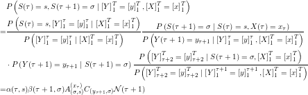
The aim of the POMDP forward-backward procedure is to find an estimator for 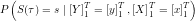 . Using Bayes’ Rule

The problem reduces thus to finding  and
and  which shall be called the forward estimate and the backward estimate respectively.
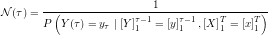
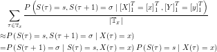
Repeated application of Bayes’ Rule and the definition of the POMDP leads to the following recursive formulation of :

This yields a recursive policy for calculating . The missing piece,  , can be calculated using the preceding recursion step for :
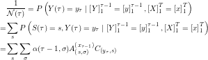
The common term of the -recursion and the  -recursion can be extracted to make the process computationally more efficient:

The result differs from the original formulation [2] merely by the fact that the appropriate transition matrix is chosen in every recursion step. It is still necessary to calculate , which can be reduced to a similar recursion:
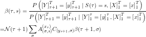
The base cases of these recursions follow directly from their probabilistic interpretation:

Using the definitions of and it is now possible to derive an unbiased estimator for . It’s definition bears a striking resemblance to the estimator derived by Devijver [2]. Analogue to the steps Baum and Welch took to derive their update rule, the need for two more probabilities arises:  and
and  . Luckily, , and again can be used to compute these probabilities.
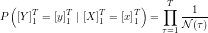
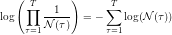
It turns out, that the values for calculated above can also be used to calculate the likelihood of the observed data under the current model parameters.
In practice the log-likelihood will be of more interest, as it’s calculation is more efficient and numerically more stable:
EM-Update Rule
The methods derived up to this point are useful to calculate state probabilities, transition probabilities and output probabilities given a model and a sequence of inputs and outputs. As Baum and Welch did in the case of HMMs, these very probabilities will now be used to derive estimators for the model’s parameters. Let  . Then
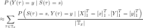
A similar scheme can be used to derive an estimator for the transition probabilities:
where 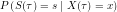 can be approximated using the above estimator (this might mean that the new estimator is biased, not quite sure about that). The result is an estimator for
  . An estimator for the output probabilities can be derived accordingly, making use of the Markov property:

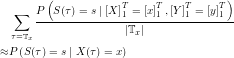
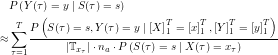
Thus,
This equation holds for every value of x. Therefore a better estimator can be derived by averaging the values over all inputs:
Implementation
To get a bit more concrete, I will add the Python code I wrote to execute the steps described above.
The definition of a POMDP. For simplicity, inputs and outputs are supposed to be natural numbers. The transition matrices corresponding to each of the input characters are stored in alist (where alist[i] is the transition matrix that corresponds to input symbol i). As before, the matrix that maps state- to observation probabilities is given by c. The initial state distribution is stored in init.
class MarkovModel(object):
    def __init__(self,alist,c,init):
        self.alist = alist
        self.c = c
        self.ns = c.shape[1]
        self.os = c.shape[0]
        self.inps = len(alist)
        self.init = init
In the above sections, the procedure was stated in a recursive form. It is, however, not advisable to actually implement the algorithm as a recursion as this will lead to a bad performance. A better approach is to use a dynamic programming approach: The and values are stored in a matrix where
- each column corresponds to one point in time

- each row corresponds to one state
This is where actually most of the magic happens.
This function will generate
- a tableau for

- a tableau for
 and
and - a tableau for

To make the computation of  and
and  more efficient, I also calculate the common factor
  as derived above:
def make_tableaus(xs,ys,m):
    alpha = np.zeros((len(ys),m.ns))
    beta  = np.zeros((len(ys),m.ns))
    gamma = np.zeros((len(ys),m.ns))
    N     = np.zeros((len(ys),1))

    # Initialize:
    gamma[0:1,:] = m.init.T*m.c[ys[0]:ys[0]+1,:]
    N[0,0] = 1 / np.sum(gamma[0:1,:])
    alpha[0:1,:] = N[0,0]*gamma[0:1,:]
    beta[len(ys)-1:len(ys),:] = np.ones((1,m.ns))

    for i in range(1,len(ys)):
        gamma[i:i+1,:] = m.c[ys[i]:ys[i]+1,:] * np.sum((m.alist[xs[i-1]].T*alpha[i-1:i,:].T),axis=0)
        N[i,0] = 1 / np.sum(gamma[i:i+1,:])
        alpha[i:i+1,:] = N[i,0]*gamma[i:i+1,:]
    for i in range(len(ys)-1,0,-1):
        beta[i-1:i] = N[i]*np.sum(m.alist[xs[i-1]]*(m.c[ys[i]:ys[i]+1,:]*beta[i:i+1,:]).T,axis=0)
    return alpha,beta,N
These tableaus can be used to solve many inference problems in POMDPs. For instance, given a sequence of inputs  and a sequence of observations
  that correspond to , estimate the probability of being in a certain state during each state. Put differently: The function
 state_estimates will calculate the posterior distribution over all latent variables.
I included an optional tableaus parameter. This ensures that, if we want to solve several inference problems, we only need to calculate the tableaus once.
def state_estimates(xs,ys,m,tableaus=None):
    if tableaus is None: tableaus = make_tableaus(xs,ys,m)
    alpha,beta,N = tableaus
    return alpha*beta
With the formulas that we derived above and using the tableaus, this becomes very simple. Note that the standard meaning of the *-operator in numpy is not matrix multiplication but element-wise multiplication.
A bit more sophisticated is the following inference problem: Given a sequence of inputs  and a sequence of observations
  that correspond to , estimate the probability of transferring between two states at each time step.
def transition_estimates(xs,ys,m,tableaus=None):
    if tableaus is None: tableaus = make_tableaus(xs,ys,m)
    alpha,beta,N = tableaus
    result = np.zeros((m.ns,m.ns,len(ys)))
    for t in range(len(ys)-1):
        a = m.alist[xs[t]]
        result[:,:,t] = a*alpha[t:t+1,:]*m.c[ys[t+1]:ys[t+1]+1,:].T*beta[t+1:t+2,:].T*N[t+1,0]
    a=m.alist[xs[len(ys)-1]]
    result[:,:,len(ys)-1] = a*alpha[-1:,:]
    return result
The next function again takes an input sequence and an output sequence and for each time step computes the posterior probability of being in a state and observing a certain output.
Note that as the sequence of outputs is already given, this function does not add much: If in time step  an output of 1 was observed, obviously the probability of observing 2 in time step will be zero.
def stateoutput_estimates(xs,ys,m,sestimate=None):
    if sestimate is None: sestimate = state_estimates(xs,ys,m)
    result = np.zeros((m.os,m.ns,len(ys)))
    for t in range(len(ys)):
        result[ys[t]:ys[t]+1,:,t] = sestimate[t:t+1,:]
    return result
Having defined these functions, we can implement the Baum-Welch style EM update procedure for POMDPs. It simply calculates
- The posterior state estimates for each

- The posterior transition estimates for each

- The posterior joint state/output estimates for each

This method can be repeated until the model converges (for some definition of convergence). The return value of this function is a new list of transition probabilities and a new matrix of output probabilities. These two define an updated POMDP model which should explain the data better than the old model.
def improve_params(xs,ys,m,tableaus=None):
    if tableaus is None: tableaus = make_tableaus(xs,ys,m)
    estimates = state_estimates(xs,ys,m,tableaus=tableaus)
    trans_estimates = transition_estimates(xs,ys,m,tableaus=tableaus)
    sout_estimates = stateoutput_estimates(xs,ys,m,sestimate=estimates)

    # Calculate the numbers of each input in the input sequence.
    nlist = [0]*m.inps
    for x in xs: nlist[x] += 1

    sstates = [np.zeros((m.ns,1)) for i in range(m.inps)]
    for t in xrange(len(ys)): sstates[xs[t]] += estimates[t:t+1,:].T/nlist[xs[t]]

    # Estimator for transition probabilities
    alist = [np.zeros_like(a) for a in m.alist]
    for t in xrange(len(ys)):
        alist[xs[t]] += trans_estimates[:,:,t]/nlist[xs[t]]
    for i in xrange(m.inps):
        alist[i] = alist[i]/(sstates[i].T)
        np.putmask(alist[i],(np.tile(sstates[i].T==0,(m.ns,1))),m.alist[i])

    c = np.zeros_like(m.c)
    for t in xrange(len(ys)):
        x = xs[t]
        c += sout_estimates[:,:,t]/(nlist[x]*m.inps*sstates[x].T)
    # Set the output probabilities to the original model if
    # we have no state observation at all.
    sstatem = np.hstack(sstates).T
    mask = np.any(sstatem == 0,axis=0)
    np.putmask(c,(np.tile(mask,(m.os,1))),m.c)

    return alist,c
How to test that? Well, we’ve seen how to calculate the log-likelihood of the data under a model:
def likelihood(tableaus):
    alpha,beta,N = tableaus
    return np.product(1/N)

def log_likelihood(tableaus):
    alpha,beta,N = tableaus
    return -np.sum(np.log(N))
Summary and Caveats
This post showed how to learn a POMDP model with python. The technique seems to be reasonably numerically stable (while I experienced major problems with a version based on the original alpha-beta method). Still there are some degeneracies that can occur, e.g. if a certain input was never observed the result of the division by nlist[xs[t]] may not be defined. That is why I used that strange mask construction to work around the problem. I do not claim that the implementation that I used is extraordinarily fast or optimised and I’d be glad about suggestions how to improve it.
I also experimented with a version of the function that creates a weighted average of the old and the new transition probabilities. This technique seemed to be more appropriate for some applications.
From a theoretical point of view the derivation I presented is no black magic at all: It turns out that learning a POMDP model is almost the same as learning a HMM, except that we have one transition matrix for each input to the system. Yet, it is still nice to see that it does work!
Finally, there is the unfortunate caveat of every EM-based technique: Even though the algorithm is guaranteed to converge, there is no guarantee that it finds the global optimum.
References
| [1] | LE Baum, T Petrie, and G Soules. A maximization technique occurring in the statistical analysis of probabilistic functions of Markov chains. The Annals of Mathematical Statistics, 1970. [ http ] |
| [2] | Pierre a Devijver. Baum’s forward-backward algorithm revisited. Pattern Recognition Letters, 3(6):369-373, December 1985. [ DOI | http ]
|
| [3] | Andrew McCallum. Overcoming incomplete perception with utile distinction memory. In Proceedings of the Tenth International Conference on Machine Learning, pages 190-196. Citeseer, 1993. [ http ]
|
| [4] | Andrew McCallum. Reinforcement learning with selective perception and hidden state. Phd thesis, University of Rochester, 1996. [ .ps.gz ] |
| [5] | Daniel Mescheder, Karl Tuyls, and Michael Kaisers. Opponent Modeling with POMDPs. In Proc. of 23nd Belgium-Netherlands Conf. on Artificial Intelligence (BNAIC 2011), pages 152-159. KAHO Sint-Lieven, Gent, 2011. [ .pdf ]
|
| [6] | Lloyd R Welch. Baum-Welch Algorithm. IEEE Information Theory Society Newsletter, 53(4), 2003. |
This file was generated by bibtex2html 1.95.

This is really interesting stuff.
Thanks so much for sharing your hard work.
Can you upload a test data set to play with as well
Cheers Mike,
I’ll try to upload some data when I find the time.
However, it is quite easy to generate some dummy data just to test how well the algorithm works yourself.
What I did is to simply created a few POMDPs and used them to sample data. Then I compared the learned model with the POMDP that I sampled the data from.
I don’t know whether there is any standard benchmark for that problem.
Hi Daniel,
I was using your code to train a POMDP .. and as i realized that I get stuck to the same probabilities if I initialize them flat (same prob to all) … but works fine when i initialize them randomly. Should this happen with this code or am i committing some mistake.
Thanks a lot,
Rahul
Hi Rahul,
Yes, that’s normal.
I suspect that this is somehow due to the “local search” nature of the algorithm.
However, I did not investigate into this phenomenon so I don’t know whether there might be a clever way around it – I indeed also ended up using random initialisation.
I hope that helps,
Daniel
and to update the initial state probabilities am I correct in updating them with the first row of apha*beta that you calculated in state_estimates function ?
Hi Daniel,
I am curious about the derivation of the whole formula. Why did you omit the influence on the transition probability by dialogue action variable? What if considering the dialogue acts space? Thanks.
-Yang
Hi Yang,
I’m afraid I don’t quite understand what your question is aiming at. The derivation above is for a generic EM-like update algorithm for a specific kind of probabilistic model (namely a POMDP).
From your comment I suspect you want to apply this model to some kind of speech recognition/NLP problem?
Cheers,
Daniel
Hi Daniel,
Thank you for your post and I found it is very helpful. I am struggling with POMDP training problem recently.
In terms of your post, I have some questions.
1. What is X and Y? Are they actions and observations?
2. When I tried to run your code, I was unable to run through. I built a POMDP with 2 states, 2 actions and 9 observations. Therefore, the state transition matrix alist was a 9*2*2 matrix, the observation matrix was a 9*2 matrix and initial state distribution was a 1*2 matrix. When the code ran to gamma[0:1,:] = m.init.T*m.c[ys[0]:ys[0]+1,:], I found that m.init.T is a 2*1 matrix and m.c[ys[0]:ys[0]+1,:] is a 1:2 matrix, thereby generating a 2*2 matrix, while gamma[0:1,:] is a 1*2 matrix. Did I build a POMDP with wrong state transition matrix, observation matrix and initial state distribution?
Thank you very much.
Regards,
Ben
Hi Ben.
I may be a little late, however, your initial state distribution should actually be for the first *observation*, not underlying state, making it a 1*9 matrix.
Hope that helps,
From Jeff
Hi Daniel,
Thank you for your post. It is very helpful.
I do not quite understand how to derive the last step in EM-Update Rule to estimate P(Y|S), Why we have to divide P(St = s, Yt = y | Y(1->T), X(1->T)) by |Tx(t)| and na (or no? I cannot see it clearly). I am wondering if you can give some clue on deriving it?
Thank you very much.
Regards,
Ben
Hi all,
we integrated some POMDP code (clean controller, file-IO for models and policies and planning algorithms) with Daniel’s learning stuff at bitbucket (see. https://bitbucket.org/bami/pypomdp/). Feel free to join us and develop the code base.
All the best
Bastian
Hi, I think I understand what Xuesong Yang was trying to say: You were talking about how one can adjust the forward-backward algorithm to POMDP but in your derivation, where it seems you wanted to show how it is done, you igonored the actions, so I think you didn’t do what you claimed you do. Also, when you introduced the notation for POMDP you actually did it for HMM.
Another thing, the POMDP model allows the observation probabilities to depend also on actions and not only on states but it seems that the implementaion you gave does not.