In this article, I want to argue that the unique properties of map data make it a particularly interesting target for techniques such as change data capture in which not only the data itself but also the changes to the data become a first-class citizen.
This article is part of a series about the specific challenges of working with map data. Part one of the series can be found here.
How Big Is A Map?
To set the stage, let us dive into one of the aspects that we have not yet considered in the previous parts of this series: How big is map data? The answer to this question is, as always, “it depends”. Nevertheless, it is possible to get a feeling for the ballpark we are playing in by looking at some numbers.
One of the data points I want to bring forward is the size of the global OSM map in pbf (protocol buffers) format which comes in at about 70GB. The size of this data loaded into a database will depend on the degree of denormalization but I would estimate the order of magnitude at a couple of hundreds of GB.
This is well below traditional Big Data territory: Traditional database systems are very well able to handle data of this scale. Nevertheless, there are a number of other considerations I would like to go into:
Firstly this scale gives us a feeling of the dimension of traditional map content: Roads, buildings, points of interest, land use information, etc. However, map data can be much more than that. A map can also include three-dimensional building models, point clouds of road-side geometries, or historical speeds per road segment. These data sets are not part of OpenStreetMap. Including them into a map data set would significantly increase its size.
Furthermore, some use cases would not only require the current snapshot of a data set but its entire history which also lands us in a territory where scaling out is a worthwhile consideration.
My final consideration is that the size of map data benefits from normalization. Consider how many streets there are that have the name “high street”. According to taginfo, in OpenStreetMap there are currently 15,354 ways with that name at the time of writing. Duplicating the string to all of these objects would require 15,354 x 11 bytes = 169kb. Pointing to one integer id of a record where this name is stored instead would require 15,354 x 4 bytes = 61kb.
For many practical applications, storing map data in a denormalized form may be necessary. In the previous article on map producers and consumers, I already noted that it is important to distinguish between runtime formats that may include use-case specific indices and store data in a denormalized fashion and exchange formats. Differences in data size are another reason to distinguish between the two.
How Is Map Data Used?
It is important to observe that map data is not static: Reality changes, new roads are constructed, restaurants close, and forests disappear. Moreover, no map is complete, and just like every other data set, map data requires continuous maintenance.
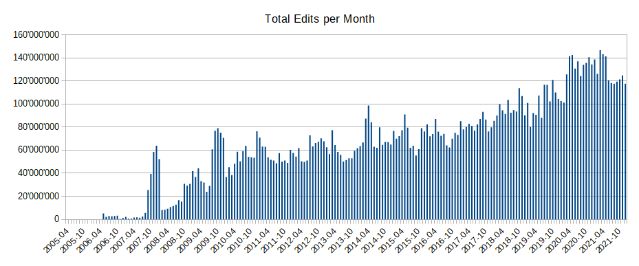
The below image shows the total number of edits per month happening on top of OpenStreetMap.
A nice way of getting an impression of how the OpenStreetMap changes is watching the edits fly by on http://osmlab.github.io/show-me-the-way/.
We have seen in an earlier article that very often the consumer of map data is another map transformation process. I also went over some typical applications of map data such as visualization, geocoding, and routing. What all of these use cases have in common is that the user typically has a question about the current state of the world. This means that most use cases will require regular maintenance of the derived data structures.
What does that mean in practice? If you are maintaining a search index to enable a geo-coding application, you probably want to update this index frequently as the underlying ground-truth data changes. If you want to display a map, this typically involves rendering the map data into a raster- or vector representation of individual tiles at different zoom levels. Again, when the underlying data changes, you have to re-render the affected tiles.
How frequently an update is required will depend on the expectations of your users. However, in general, the faster the map is updated, the quicker it includes improvements and the closer it reflects reality.
The data size analysis we went over above shows that it is absolutely feasible to update derived map data in batches by reprocessing the global database. However, this is also incredibly wasteful: Assuming you want to update your derived data relatively frequently, most of the map will not have changed between two updates.
Indeed, OpenStreetMap statistics suggest that we can currently expect 2-3 edits per minute on average. If we could simply propagate these edits to your derived index instead of re-processing the entire map, it would appear easy to keep the derived data up-to-date with only minimal delay.
How OpenStreetMap Handles Change Data
The most common way of capturing change data in OpenStreetMap is the osmChange format, often shipped in the form of .osc files.
The osmChange format captures the state of each changed node/way/relation after modification. Here is an example of what this looks like. In the changeset with ID 120397146, the OSM user Marek-M edited a morgue in Argentina and a part of a nordic skiing route in Norway:
<osmChange version="0.6" generator="CGImap 0.8.6 (2584511 spike-08.openstreetmap.org)" copyright="OpenStreetMap and contributors" attribution="http://www.openstreetmap.org/copyright" license="http://opendatacommons.org/licenses/odbl/1-0/">
    <modify>
        <node id="9696061597" visible="true" version="3" changeset="120397146" timestamp="2022-04-30T19:20:35Z" user="Marek-M" uid="598860" lat="-27.3312386" lon="-55.0495604">
            <tag k="addr:postcode" v="3362"/>
            <tag k="addr:street" v="Colón"/>
            <tag k="amenity" v="mortuary"/>
            <tag k="description" v="SALON VELATORIO COOP. ELECTRICA DE AGUA POTABLE"/>
        </node>
    </modify>
    <modify>
        <way id="1055835542" visible="true" version="3" changeset="120397146" timestamp="2022-04-30T19:20:35Z" user="Marek-M" uid="598860">
            <nd ref="251867280"/>
            <nd ref="2645448819"/>
            <nd ref="2645448820"/>
            <nd ref="2645448824"/>
            <nd ref="9701595105"/>
            <tag k="description" v="Attention: Very steep section! (2022-03-18, Seuche)"/>
            <tag k="leisure" v="track"/>
            <tag k="name" v="Panoramaløypa lang"/>
            <tag k="piste:difficulty" v="intermediate"/>
            <tag k="piste:grooming" v="classic+skating"/>
            <tag k="piste:type" v="nordic"/>
            <tag k="route" v="piste"/>
            <tag k="source" v="own survey (2022-03-18), Seuche"/>
            <tag k="type" v="route"/>
            <tag k="website" v="https://skeikampen.no/aktiviteter/vinter/langrenn/"/>
        </way>
    </modify>
</osmChange>
A number of things are interesting to note about this format. The first noteworthy aspect is the fact that this format does not show exactly what changed between the two versions. Getting the entire new state of a map feature is a design choice that makes certain operations slightly easier and other operations slightly harder.
Consider a program that consumes the stream of OSM changes to keep track of the count of objects tagged with highway that also have a surface tag. The osmChange format makes this easy as it allows you to only keep track of the running count. You do not need to keep the entire current state of the map. Without the additional context that osmChange provides, whenever you receive a change to a surface tag, you would have had to look up in a local state of the map whether that same object also has a highway tag.
Consider on the other hand an application that prioritizes the re-rendering of an object giving higher priority to highly visible modifications like turning an admin_level 4 into an admin_level 2. This is something that you cannot determine just by looking at the osmChange file because you can’t tell which of the tags are different between the two versions. To solve this issue, you would need to locally keep track of the relevant state (e.g. all objects that have an admin_level) to compute the difference.
The second observation is, that it is not always that obvious to see when an object’s geometry has changed. When the osmChange data contains a node geometry modification, this does not tell you anything about ways that contain this node. If your application needs to be notified whenever a road geometry changes, you need to keep track of the nodes defining each road and react whenever you see a change to one of these nodes. Similarly, changes to members of a relation will not result in a remark that this relation has changed in the osmChage file.
Luckily, in practice, there are several very easy-to-use tools that the OSM community has built over the years to work with osc files. Assume, for example, that you need to keep track of some data derived from OSM in a Postgres database. Chances are that osm2pgsql will fit that use case. With this tool, you can define the format of the derived data as a function of the input map in a lua script. For example, if you are interested in all geometries of features annotated with the highway tag, you could express this as follows:
local tables = {}
tables.highways= osm2pgsql.define_way_table('highways', {
    { column = 'geom', type = 'linestring' },
})
function osm2pgsql.process_way(object)
    if object.tags.highway then
        tables.highways:add_row({})
    end
end
What is particularly nice about osm2pgsql is that it can deal with osc files out of the box: Once the database has been initialized once from a full dump of the data, your derived dataset can be kept up to date simply by running the same osm2pgsql command on the osc file that contains the update.
The architecture of the OpenStreetMap system relies heavily on such techniques. The original model of OSM data is not really practical for rendering, for example. As we saw earlier when we considered map data consumers, it is often necessary to transform map data into a format more adapted to the use case at hand. Osm2pgsql can denormalize geometries, making the setup of a rendering pipeline much easier.

Context
Let us take a step back and think more generally about change data processing. As such, processing change data seems simple. Naively it would seem tempting to think about this as a stream-processing problem in which each map update triggers a function call with the update data in its input which would then map this input change to whatever output change is required (e.g. an index update).
If your use case is a text-based search index, that may very well work out as you might update the index purely with the information on the changed object.
In practice, as we have seen above, most updates require a bit more than the information on what has changed. Most of the time you will require context.
Consider what would change in the above example if you also wanted to store the country that an object is located in to enable queries like “MacDonalds in Germany”. Now you will have to do a spatial or referential lookup in the set of all countries for a given change. You will also have to invalidate a part of the index if ever a country’s geometry changes. (Contrary to what you might think, this does happen from time to time.)
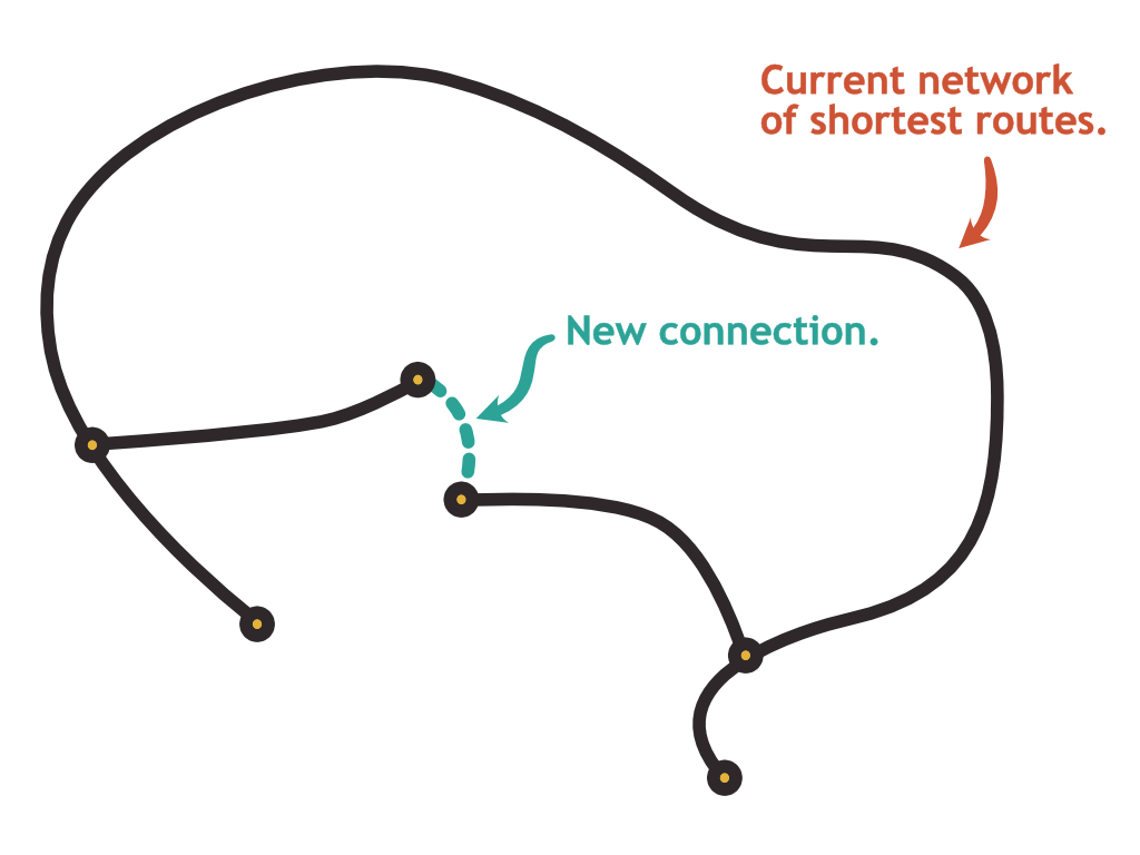
The situation gets even more complex if the derived data you maintain is a contraction hierarchy index. Such an index is basically a list of pre-calculated routes. A newly added road element can in theory invalidate routes that are not even close to that new element as shown in the image below. You will probably have to keep track of the road network as context information and be smart about invalidating the right nodes in your hierarchy.
We can conclude that most processes listening to map changes will fall into the category of stateful stream processing. The state that needs to be stored depends on the operation that needs to be performed.
Order
An important question in the stream processing design space is whether or not the order of events is significant. If your process can tolerate out-of-order events and late arrivals, scaling the system is easier because you can partition the queues containing the incoming events.
Processing map change data as described above resembles what is commonly known as change data capture. It is very common for change data capture applications to be sensitive to the ordering of events as later events frequently depend on earlier events. I found the same to be true for many map data processing use cases.
Luckily, in the case of OpenStreetMap, this is not a big issue as the frequency of changes is so low that scalability is not an issue. It is quite reasonable to run osm2pgsql to apply osmChange files in sequence.
Conclusion
We have seen that map data is often consumed by another transformation process. Furthermore, as the size of a change to the map is usually significantly smaller than the size of the map itself, we noticed that there is a lot of benefit in looking at this process as a stateful stream processing problem, making change data a first-class citizen.
As we have seen, the tools that the OpenStreetMap community has developed over the years are adapted to this reality. These tools are central to the OSM architecture and it is absolutely feasible to use them to keep your own derived data up to date.
